Making birds fly

solution

Date

23 April 2024

1. The `Bird` object

Our blueprint for Birds looks like this. Notice that we declare it to be mutable – when a Bird flies, its position coordinates must change.

mutable struct Bird
  x::Float64
  y::Float64
  dir_x::Float64
  dir_y::Float64
end

2. The population

To create a population of Birds, it is easiest to use an array comprehension. Notice how we use the rand() function to give each bird a random position and random direction. (The number of birds in the population wasn’t specified in the homework assignment – my mistake. Here, I’ve decided to create 10 birds.)

population = [Bird(rand(), rand(), rand(), rand()) for i in 1:10]

10-element Vector{Bird}:
 Bird(0.521213795535383, 0.5868067574533484, 0.8908786980927811, 0.19090669902576285)
 Bird(0.5256623915420473, 0.3905882754313441, 0.044818005017491114, 0.933353287277165)
 Bird(0.5805599818745412, 0.32723787925628356, 0.5269959187969865, 0.8362285750521512)
 Bird(0.04090613602769255, 0.4652015053812224, 0.3626493264184424, 0.10220460648875951)
 Bird(0.7201025594903295, 0.5736192424686392, 0.6644684787269287, 0.29536650475479964)
 Bird(0.2765974461749666, 0.9834357111198399, 0.8808974908158065, 0.23401680577405504)
 Bird(0.3809493792861086, 0.13194373253949954, 0.08829101913227844, 0.31350491450772877)
 Bird(0.4636097443249143, 0.7136359224862079, 0.20592490948670994, 0.09055116421778064)
 Bird(0.5819123423876457, 0.3114475007050529, 0.12114752051812694, 0.20452981732035946)
 Bird(0.38669016290895364, 0.018571999589938493, 0.07218072370140682, 0.9142465859437933)

3. Sourcing the plotting code

We now include the source code in the file plot_birds.jl which allows us to plot the population. (I store my scripts in a folder named jl in the parent directory of the current working directory, hence the ../jl/ construction before the filename.) Since this code requires the presence of the Plots package, we also first load that package using using.

using Plots
include("../jl/plot_birds.jl")

4. Plotting the population

We can now plot:

plot(population)

Why are all our birds pointing in more or less the same direction? Recall that we used rand() to initialize the birds’ positions and directions, and recall that rand() returns a random number between 0 and 1. But we can also quite easily generate a random float between -1 and 1; see:

[2*rand() - 1 for i in 1:10]

10-element Vector{Float64}:
 -0.22525187549286851
  0.5438327116895545
 -0.24523348113449273
  0.7511099991192371
 -0.4708637192761387
  0.8037546490608298
  0.7293861840623399
  0.4644763024359402
 -0.7936063069983399
  0.1751698724177022

With this idea in mind, let’s re-initialize our population:

population = [Bird(2*rand() - 1, 2*rand() - 1, 2*rand() - 1, 2*rand() - 1) for i in 1:10]

10-element Vector{Bird}:
 Bird(0.618865511882924, -0.5523183945589438, 0.7170489219693619, -0.24916615259097208)
 Bird(0.3534141180790922, 0.8417688482534209, 0.4129222831361803, 0.3919753816200593)
 Bird(0.7579538838754145, -0.16543176889487166, -0.12700639607293884, -0.6063073498246891)
 Bird(0.17059453226859533, 0.12660681452801836, -0.07117384268707516, 0.6495748680565732)
 Bird(0.1591833330768717, 0.6077337180274938, 0.08377142581999197, 0.5523786724183681)
 Bird(-0.8566393842375593, 0.8653672763283604, 0.6817832906156263, 0.590731985726523)
 Bird(0.5890138703978984, 0.280887894872357, -0.10813826831817863, -0.9059532971107356)
 Bird(0.2775156760816275, 0.41475391462741396, 0.9860955611224076, -0.6907174051634926)
 Bird(-0.7656879482170376, -0.8057846770570476, -0.8824796694661512, 0.24197793679586144)
 Bird(0.3464419510792771, -0.4091392851668356, 0.2423652677929784, -0.33347994991774543)

And plot it:

plot(population)

Note

Clearly my plotting code has a bug in it: look at the four birds which have arrows pointing to them rather than away from them. (This is because when writing the code, I only tested it with birds that had positive positions and positive directions… important lesson to be learned here: when deploying code, especially code for other people to use, always test it under all imaginable circumstances!) We’ll ignore this little problem for now. A patched version of the plotting code is provided at the end of this solution.

5. The `fly!` function

We now get to the meat of the exercise: making these birds fly. The instruction was to

move x in the direction of dir_x by a little amount – let’s call that little amount delta – and […] move y in the direction of dir_y by the same amount.

How do we do this?

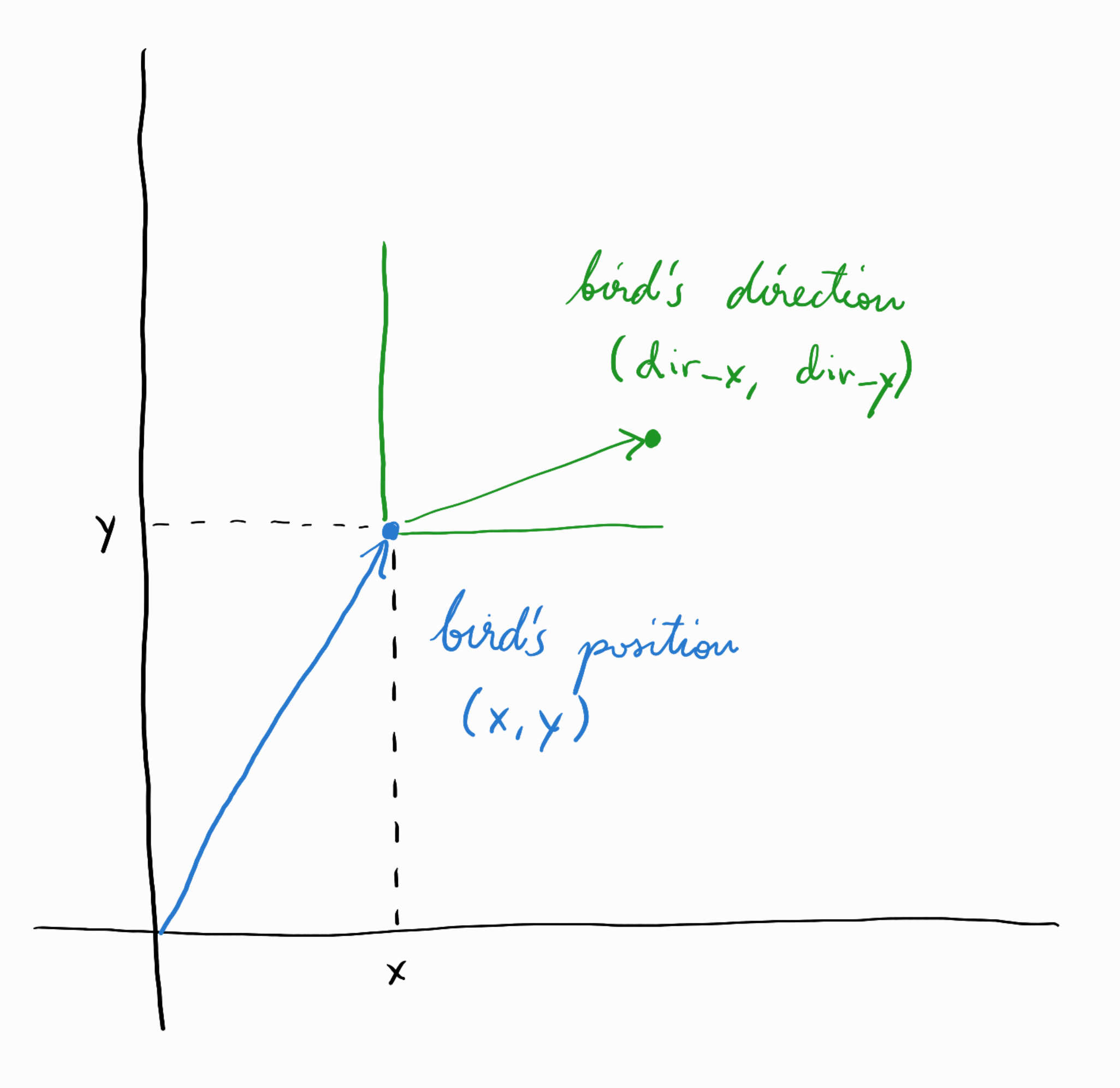
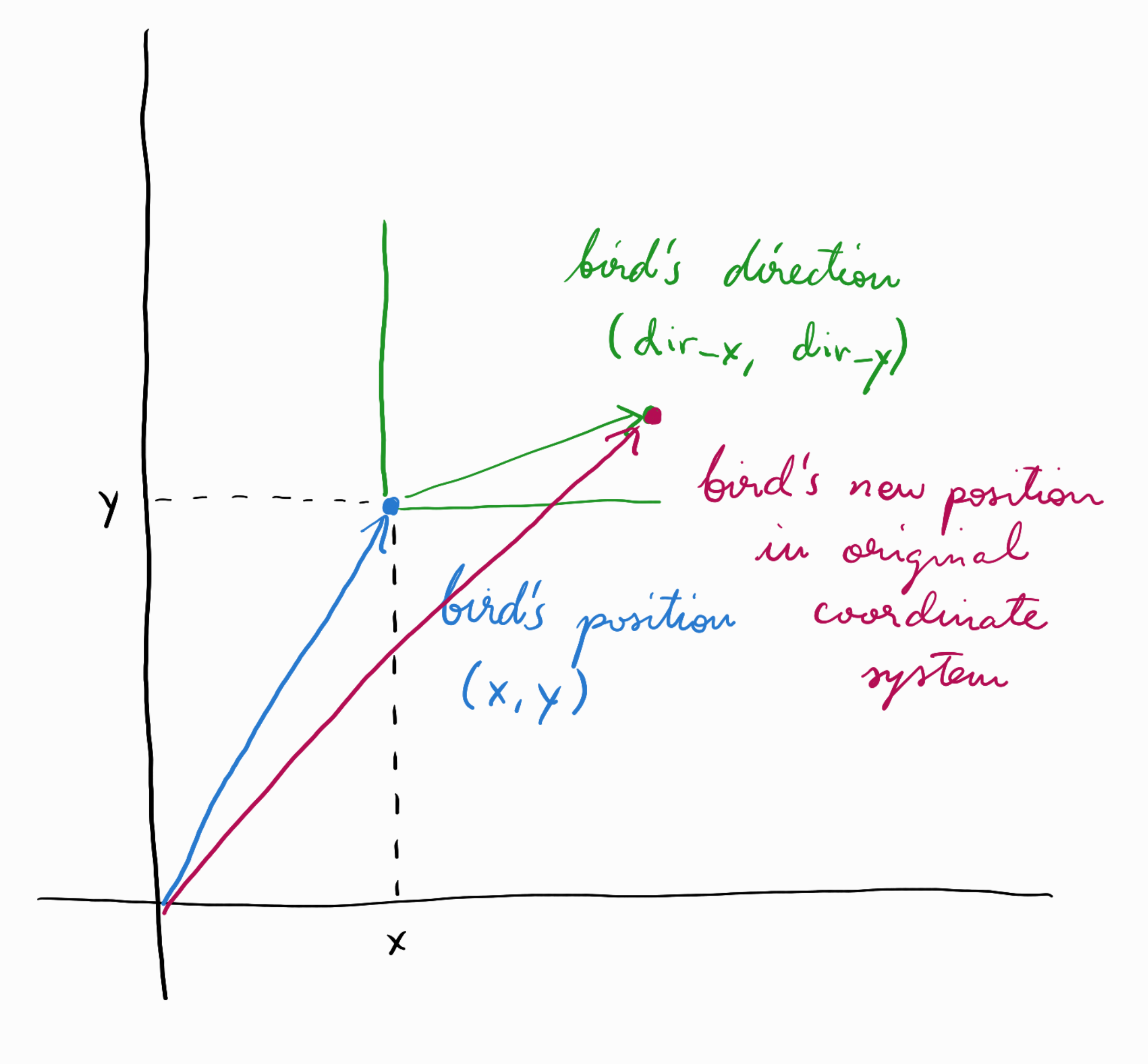
One way is to imagine that dir_x and dir_y define a local coordinate system – local to the bird. (In fact, this is what my plotting code implicitly does in order to draw the direction arrows.) Hence, for example, if dir_x is 0 and dir_y is 1, this would mean that the bird is pointing directly northwards. You can then think of the bird’s position as a vector, an arrow from the origin (0,0) to (x,y), and you can similarly think of the birds’s direction as a vector, an arrow from (x,y) to (dir_x, dir_y); see this illustration:

To make the bird move from (x,y) for (dir_x, dir_y), we perform vector summation: we set the new value of x to be x + dir_x and the new value of y to be y + dir_y.

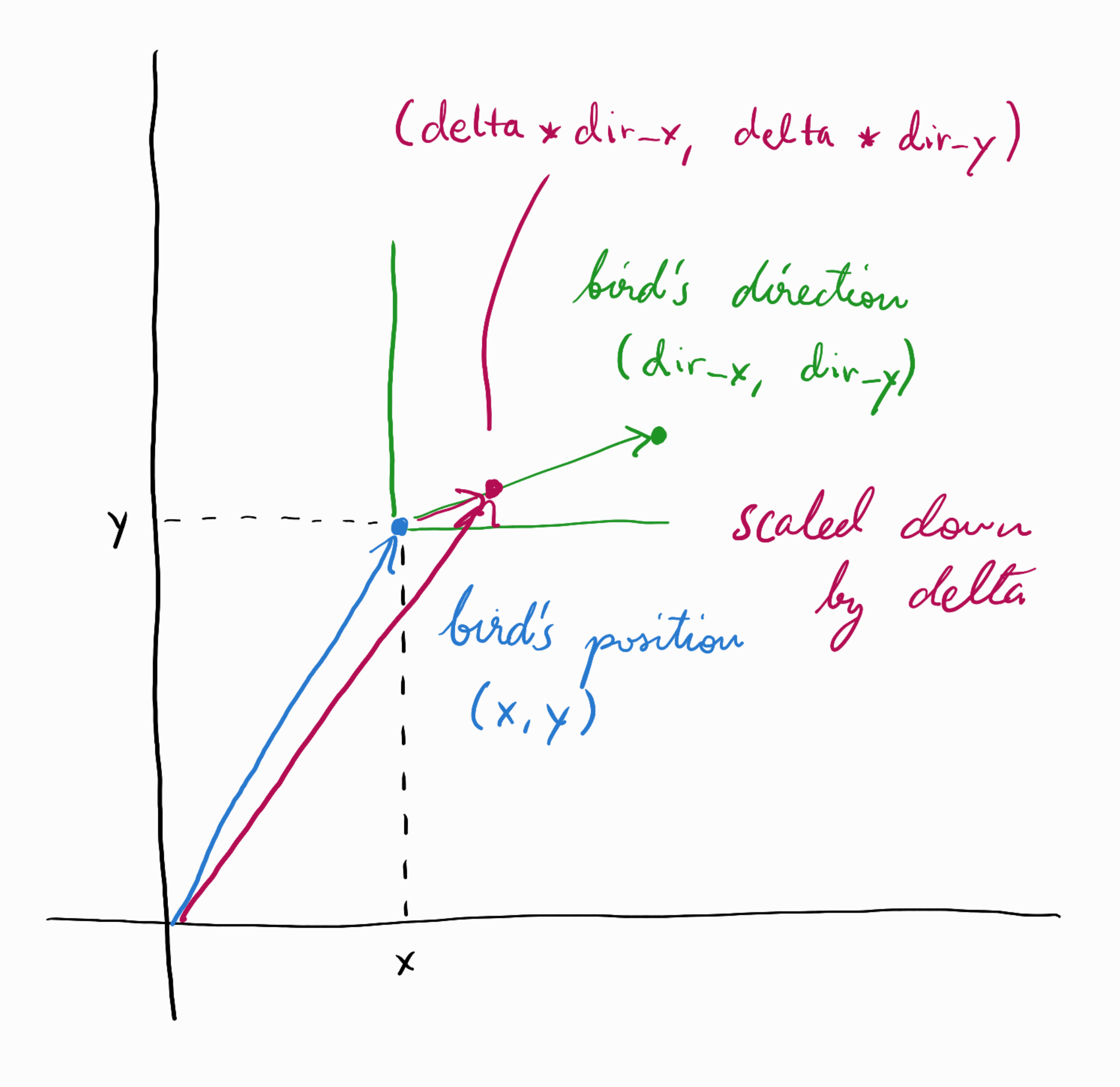
The only thing that remains is that “little amount delta”. If we replace the direction vector (dir_x, dir_y) with (delta*dir_x, delta*dir_y), then we are effectively scaling it down (assuming delta has a value between 0 and 1):

Putting all of the above together, we can now define our function for flying a bird:

function fly!(b::Bird, delta::Float64)
  b.x = b.x + delta*b.dir_x
  b.y = b.y + delta*b.dir_y
end

fly! (generic function with 1 method)

Simple! (In fact, this is the usual state of affairs: writing the code itself is not so difficult, the difficult thing is the thinking that has to be done first…)

6. Testing

Let’s now finally test the fly! function. This is what our population looked like initially:

plot(population)

Let’s now apply fly! to the first bird in the population a few times. (I’m choosing a very large value for delta so that we see the effects more clearly.)

delta = 0.9
fly!(population[1], delta)
fly!(population[1], delta)
fly!(population[1], delta)

-1.2250670065545686

Note

What is this number that is returned? Recall that Julia functions automatically return the results of the last expression evaluated inside a function body, in this case, the value of b.y. If you want to disable this, add return nothing as the last line of your function definition, like this:

function fly!(b::Bird, delta::Float64)
  b.x = b.x + delta*b.dir_x
  b.y = b.y + delta*b.dir_y
  return nothing
end

Let’s see what happened:

plot(population)

One bird is flying away from the population, in the direction of its direction arrow, exactly as expected.

Bonus: making the entire population fly

Recall that in Julia, functions can be broadcast over arrays, meaning the function gets applied elementwise to each element of the array. Since our population of birds is an array, we can now very easily make each bird fly:

fly!.(population, 0.9)
plot(population)

Furthermore, we can use an array comprehension to make each bird fly some specified number of times. For example here 20 times:

[fly!.(population, 0.1) for t in 1:20]
plot(population)

Updated plotting code

There are really three problems with the code in plot_birds.jl:

Sometimes the direction arrow points towards the bird rather than away from it, as expected.
When the birds have flown numerous times, the direction arrows become so small that they can barely be seen (cf. the above population plot).
Finally, I forgot to include a line in the code that specifies that the presence of the Plots package is required, leading to error messages in case the end-user hasn’t loaded Plots before attempting to use the code.

I have fixed these problems in an updated plot_birds_fixed.jl script which you can download here.

Applied to our population’s current state, the bug-fixed plotting code now gives:

include("../jl/plot_birds_fixed.jl")
plot(population)

Looks much better, doesn’t it?

Other Formats

1. The Bird object